Tutorial 1: Standard REXEE simulations

In this tutorial, we will demonstrate how one can use the different command-line interfaces (CLIs) implemented in the Python package ensemble_md to prepare, perform, and analyze a REXEE simulation to estimate the solvation free energy of a toy molecule composed of 4 interaction sites. For a more comprehensive understanding, we strongly recommend reading our documentation on launching REXEE simulations before starting this tutorial. For the theory behind the REXEE method, we recommend reading our JCTC paper or the theory section of our documentation.

To run this tutorial, you will need different setups depending on your computing environment:

• You can simply click the “launch binder” badge above to run this tutorial on Binder without installing anything.

• If you prefer to run this tutorial locally, either on you laptop, workstation, or an HPC cluster, you will need to install the following software:

  • GROMACS (version 2022.5 or later)

  • ensemble_md (version 1.0.0 or later)

Additionally, you will need to have MPI launcher commands (e.g., mpirun or mpiexec) installed on your system to run the GROMACS simulations in parallel. You will need at least four CPU cores to run the simulation in this tutorial. (You can execute nproc in the terminal to check the number of CPU cores on your system.)

Notably, this tutorial assumes that you understand the basics of the expanded ensemble (EE) method and relevant simulation parameters in GROMACS. If not, we recommend reading the this tutorial or the following GROMACS documentation pages:

• A very brief description about the expanded ensemble method

• Relevant MDP parameters in GROMACS, especially the section of free energy calcualtion and the section of expanded ensemble calculations.

0. Background knowledge: A two-stage protocol

In methods such as expanded ensembles or REXEE, where each alchemical state has an associated weight (see here), it is common to use a two-stage protocol for alchemical free energy calculations. Specifically, this protocol is composed of the following two stages:

• A weight-updating stage: In a weight-updating stage, the weights of different states are constantly updated until convergence during the simulation, usually by methods such as the Wang-Landau algorithm or its \(1/t\) variant. The purpose of this stage is to obtain weights that could flatten out the free energy surface along the alchemical direction such that all states have a roughly equal chance to be visited in the next stage, i.e., the fixed-weight stage.

• A fixed-weight stage: In a fixed-weight stage, the weights of different alchemical states are fixed at predefined values usually converged in a weight-updating stage. Unlike weight-updating simulations, a fixed-weight simulation is in equilibrium, from which the potential energy data can be analyzed by free energy estimators that require equilibrium data for free energy calculations, such as TI, BAR, MBAR, etc.

With this protocol, one can use a weight-updating EE/REXEE simulation followed by a fixed-weight EE/REXEE simulation to perform free energy calculations. In our paper, we have compared EE and REXEE methods in both weight-updating and fixed-weight phases comprehensively.

Notably, this tutorial will only focus on fixed-weight REXEE simulations, with the weights provided by a weight-updating EE simulation not shown here. If you are interested in using a weight-updating REXEE simulation to obtain alchemical weights to seed a fixed-weight simulation, you can simply adopt the workflow for running fixed-weight REXEE simulations introduced in this tutorial, with input MDP files replaced by the ones for weight-updating EE simulations.

1. Preparing simulation inputs for a REXEE simulation

As mentioned in our documentation, running a REXEE simulation at least requires the following four input files:

• One YAML file that specifies REXEE parameters.

• One GROMACS GRO file of the system of interst.

• One GROMACS TOP file of the system of interst.

• One GROMACS MDP template for customizing MDP files for different replicas during the simulation.

In the folder where this tutorial resides (docs/examples/tutoria_1 in the repository), you should find all these necessary input files, including params.yaml, sys.gro, sys.top, and expanded.mdp. Note that the file example_outputs.zip is not relevant until the third section (Analyzing a REXEE simulation).

!ls

example_outputs.zip  params.yaml           sys.gro
expanded.mdp         standard_REXEE.ipynb  sys.top

While you could use multiple GRO and TOP files, one for each replica in a REXEE simulation, in this tutorial, we will use the same GRO and TOP files for all replicas to keep the demonstration straightforward. As for the MDP template expanded.mdp, it can be inspected that it adopts common/typical settings for a fixed-weight EE simulation, since here our goal is to set up a fixed-weight REXEE simulation. In the MDP template, it can also be seen that 9 alchemical intermediate states are defined to decouple van der Waals and coulombic interactions.

During the REXEE simulation, customized MDP files will be generated for different replicas such that the MDP file for each replica only considers the set of states that the replica is constrained to. Notably, the weights specified via the MDP parameter init_lambda_weights were obtained from a weight-updating EE simulation. If you would like to run a weight-updating REXEE simulation, simply use an MDP file for running a weight-updating EE simulation, i.e., and MDP file without init_lambda_weights being specified, and with options such as wl_scale, wl_ratio, init_wl_delta, lmc_stats, lmc_weights_equil, weight_equil_wl_delta specified.

Now, with these three GROMACS inputs prepared, let’s briefly review the input YAML file that specifies REXEE parameters. (For detailed information about all possible parameters that can be specified in the YAML file, please refer to our documentation.)

!cat params.yaml

# Simulation parameters
gmx_executable: 'gmx'
gro: sys.gro
top: sys.top
mdp: expanded.mdp
n_sim: 4
n_iter: 5
s: 1
nst_sim: 500
runtime_args: {'-nt': '1'}

# Data analysis parameters
free_energy: True

As a minimum working example, this YAML file only specifies the compulsory simulation parameters and adopts default values for all optional parameters, execpt that runtime_args is specified to run each EE replica using one thread (-nt 1) for a reasonable simulation performance. Notably, Binder should have 72 cores by default (as can be checked by nproc), but using -nt 1 is much faster than using other values for this toy system. If you are not using Binder but your own local machine or an HPC cluster, you may want to try out other -nt values to ensure reasonable performance.

In our case, we will run our a REXEE simulation composed of 4 replicas, with each replica performed with one thread (-nt 1). With the total number of states as 9 and a state shift of 1, this means that replicas 0, 1, 2, 3 are constrained to sampling states 0-5, 1-6, 2-7, and 3-8, respectively. The simulation will attempt to swap coordinates between replicas every 500 integration steps, and perform 5 iterations in total. (Note that generally we need a much larger number of iterations. Here we use a very small value just for demosntration purposes.)

If you are interested in trying out other numbers of replicas or state shifts given 9 alchemical intermediate states, you can use the CLI explore_REXEE to enumerate all possible REXEE configurations.

!explore_REXEE -N 9

Exploration of the REXEE parameter space
=======================================
[ REXEE parameters of interest ]
- N: The total number of states
- r: The number of replicas
- n: The number of states for each replica
- s: The state shift between adjacent replicas

[ Solutions ]
- Solution 1: (N, r, n, s) = (9, 2, 5, 4)
  - Replica 0: [0, 1, 2, 3, 4]
  - Replica 1: [4, 5, 6, 7, 8]

- Solution 2: (N, r, n, s) = (9, 2, 6, 3)
  - Replica 0: [0, 1, 2, 3, 4, 5]
  - Replica 1: [3, 4, 5, 6, 7, 8]

- Solution 3: (N, r, n, s) = (9, 2, 7, 2)
  - Replica 0: [0, 1, 2, 3, 4, 5, 6]
  - Replica 1: [2, 3, 4, 5, 6, 7, 8]

- Solution 4: (N, r, n, s) = (9, 2, 8, 1)
  - Replica 0: [0, 1, 2, 3, 4, 5, 6, 7]
  - Replica 1: [1, 2, 3, 4, 5, 6, 7, 8]

- Solution 5: (N, r, n, s) = (9, 3, 5, 2)
  - Replica 0: [0, 1, 2, 3, 4]
  - Replica 1: [2, 3, 4, 5, 6]
  - Replica 2: [4, 5, 6, 7, 8]

- Solution 6: (N, r, n, s) = (9, 3, 7, 1)
  - Replica 0: [0, 1, 2, 3, 4, 5, 6]
  - Replica 1: [1, 2, 3, 4, 5, 6, 7]
  - Replica 2: [2, 3, 4, 5, 6, 7, 8]

- Solution 7: (N, r, n, s) = (9, 4, 3, 2)
  - Replica 0: [0, 1, 2]
  - Replica 1: [2, 3, 4]
  - Replica 2: [4, 5, 6]
  - Replica 3: [6, 7, 8]

- Solution 8: (N, r, n, s) = (9, 4, 6, 1)
  - Replica 0: [0, 1, 2, 3, 4, 5]
  - Replica 1: [1, 2, 3, 4, 5, 6]
  - Replica 2: [2, 3, 4, 5, 6, 7]
  - Replica 3: [3, 4, 5, 6, 7, 8]

- Solution 9: (N, r, n, s) = (9, 5, 5, 1)
  - Replica 0: [0, 1, 2, 3, 4]
  - Replica 1: [1, 2, 3, 4, 5]
  - Replica 2: [2, 3, 4, 5, 6]
  - Replica 3: [3, 4, 5, 6, 7]
  - Replica 4: [4, 5, 6, 7, 8]

- Solution 10: (N, r, n, s) = (9, 6, 4, 1)
  - Replica 0: [0, 1, 2, 3]
  - Replica 1: [1, 2, 3, 4]
  - Replica 2: [2, 3, 4, 5]
  - Replica 3: [3, 4, 5, 6]
  - Replica 4: [4, 5, 6, 7]
  - Replica 5: [5, 6, 7, 8]

- Solution 11: (N, r, n, s) = (9, 7, 3, 1)
  - Replica 0: [0, 1, 2]
  - Replica 1: [1, 2, 3]
  - Replica 2: [2, 3, 4]
  - Replica 3: [3, 4, 5]
  - Replica 4: [4, 5, 6]
  - Replica 5: [5, 6, 7]
  - Replica 6: [6, 7, 8]

- Solution 12: (N, r, n, s) = (9, 8, 2, 1)
  - Replica 0: [0, 1]
  - Replica 1: [1, 2]
  - Replica 2: [2, 3]
  - Replica 3: [3, 4]
  - Replica 4: [4, 5]
  - Replica 5: [5, 6]
  - Replica 6: [6, 7]
  - Replica 7: [7, 8]

If you want to list all possible configurations that use 4 replicas for sampling 9 alchemical states, you can further specify the number of replicas via the flag -r:

!explore_REXEE -N 9 -r 4

Exploration of the REXEE parameter space
=======================================
[ REXEE parameters of interest ]
- N: The total number of states
- r: The number of replicas
- n: The number of states for each replica
- s: The state shift between adjacent replicas

[ Solutions ]
- Solution 1: (N, r, n, s) = (9, 4, 3, 2)
  - Replica 0: [0, 1, 2]
  - Replica 1: [2, 3, 4]
  - Replica 2: [4, 5, 6]
  - Replica 3: [6, 7, 8]

- Solution 2: (N, r, n, s) = (9, 4, 6, 1)
  - Replica 0: [0, 1, 2, 3, 4, 5]
  - Replica 1: [1, 2, 3, 4, 5, 6]
  - Replica 2: [2, 3, 4, 5, 6, 7]
  - Replica 3: [3, 4, 5, 6, 7, 8]

For more information about the flags available for explore_REXEE, please run explore_REXEE -h/explore_REXEE --help and read the help message. For rules of thumb about specifying the configurational parameters (including the number of states, number of replicas, state shift and swapping frequency), please refer to our documentation or paper.

2. Performing a REXEE simulation

With all the input files in place, we can now run a fixed-weight REXEE simulation using the CLI run_REXEE with the command shown in the cell below.

If you are using a laptop with 4 CPU cores, this may take around 15 minutes to complete. If you run the tutorial on Binder, this should take around 3 minutes. Note that here we use default values for all flags of the CLI run_REXEE. For more information about the flags, please run run_REXEE -h/run_REXEE --help and read the help message.

!mpirun -np 4 run_REXEE

Current time: 01/08/2024 08:49:27
Command line: /srv/conda/envs/notebook/bin/run_REXEE

Important parameters of REXEE
=============================
Python version: 3.10.14 | packaged by conda-forge | (main, Mar 20 2024, 12:45:18) [GCC 12.3.0]
GROMACS executable: /srv/conda/envs/notebook/bin.AVX2_256/gmx
GROMACS version: 2023.3-conda_forge
ensemble_md version: 0.9.0+177.g9f48c4c.dirty
Simulation inputs: sys.gro, sys.top, expanded.mdp
Verbose log file: True
Proposal scheme: exhaustive
Whether to perform weight combination: False
Type of means for weight combination: simple
Whether to perform histogram correction: False
Histogram cutoff for weight correction: -1
Number of replicas: 4
Number of iterations: 5
Length of each replica: 1.0 ps
Frequency for checkpointing: 100 iterations
Total number of states: 9
Additionally defined swappable states: None
Additional grompp arguments: None
Additional runtime arguments: {'-nt': '1'}
External modules for coordinate manipulation: None
MDP parameters differing across replicas: None
Alchemical ranges of each replica in REXEE:
  - Replica 0: States [0, 1, 2, 3, 4, 5]
  - Replica 1: States [1, 2, 3, 4, 5, 6]
  - Replica 2: States [2, 3, 4, 5, 6, 7]
  - Replica 3: States [3, 4, 5, 6, 7, 8]

Iteration 0:  0.0 -  1.0 ps
===========================
Generating TPR files ...
Running EXE simulations ...

Below are the final states being visited:
  Simulation 0: Global state 3
  Simulation 1: Global state 4
  Simulation 2: Global state 3
  Simulation 3: Global state 6

Parsing ./sim_0/iteration_0/md.log ...
Parsing ./sim_1/iteration_0/md.log ...
Parsing ./sim_2/iteration_0/md.log ...
Parsing ./sim_3/iteration_0/md.log ...

Swappable pairs: [(0, 1), (0, 2), (1, 2), (1, 3), (2, 3)]

Proposed swap: (1, 3)
  Proposing a move from (x^i_m, x^j_n) to (x^i_n, x^j_m) ...
  U^i_n - U^i_m = 6.26 kT, U^j_m - U^j_n = 525.23 kT, Total dU: 531.49 kT
  Acceptance rate: 0.000 / Random number drawn: 0.715
  Swap rejected!
  Current list of configurations: [0, 1, 2, 3]

Remaining swappable pairs: [(0, 2)]

Proposed swap: (0, 2)
  Proposing a move from (x^i_m, x^j_n) to (x^i_n, x^j_m) ...
  U^i_n - U^i_m = 0.00 kT, U^j_m - U^j_n = 0.00 kT, Total dU: 0.00 kT
  Acceptance rate: 1.000 / Random number drawn: 0.630
  Swap accepted!
  Current list of configurations: [2, 1, 0, 3]

The finally adopted swap pattern: [2, 1, 0, 3]
The list of configurations sampled in each replica in the next iteration: [2, 1, 0, 3]
Note: No weight correction will be performed.
Note: No weight combination will be performed.

  The alchemical weights of all states:
  [0.0, 1.613, 2.714, 3.409, 3.604, 4.785, 5.38, 3.298, 0.363]

Iteration 1:  1.0 -  2.0 ps
===========================
Generating TPR files ...
Running EXE simulations ...

Below are the final states being visited:
  Simulation 0: Global state 3
  Simulation 1: Global state 2
  Simulation 2: Global state 4
  Simulation 3: Global state 4

Parsing ./sim_0/iteration_1/md.log ...
Parsing ./sim_1/iteration_1/md.log ...
Parsing ./sim_2/iteration_1/md.log ...
Parsing ./sim_3/iteration_1/md.log ...

Swappable pairs: [(0, 1), (0, 2), (0, 3), (1, 2), (2, 3)]

Proposed swap: (1, 2)
  Proposing a move from (x^i_m, x^j_n) to (x^i_n, x^j_m) ...
  U^i_n - U^i_m = -0.14 kT, U^j_m - U^j_n = 0.57 kT, Total dU: 0.43 kT
  Acceptance rate: 0.650 / Random number drawn: 0.407
  Swap accepted!
  Current list of configurations: [2, 0, 1, 3]

Remaining swappable pairs: [(0, 3)]

Proposed swap: (0, 3)
  Proposing a move from (x^i_m, x^j_n) to (x^i_n, x^j_m) ...
  U^i_n - U^i_m = 0.71 kT, U^j_m - U^j_n = -0.78 kT, Total dU: -0.07 kT
  Acceptance rate: 1.000 / Random number drawn: 0.590
  Swap accepted!
  Current list of configurations: [3, 0, 1, 2]

The finally adopted swap pattern: [3, 2, 1, 0]
The list of configurations sampled in each replica in the next iteration: [3, 0, 1, 2]
Note: No weight correction will be performed.
Note: No weight combination will be performed.

  The alchemical weights of all states:
  [0.0, 1.613, 2.714, 3.409, 3.604, 4.785, 5.38, 3.298, 0.363]

Iteration 2:  2.0 -  3.0 ps
===========================
Generating TPR files ...
Running EXE simulations ...

Below are the final states being visited:
  Simulation 0: Global state 5
  Simulation 1: Global state 3
  Simulation 2: Global state 4
  Simulation 3: Global state 6

Parsing ./sim_0/iteration_2/md.log ...
Parsing ./sim_1/iteration_2/md.log ...
Parsing ./sim_2/iteration_2/md.log ...
Parsing ./sim_3/iteration_2/md.log ...

Swappable pairs: [(0, 1), (0, 2), (1, 2), (1, 3), (2, 3)]

Proposed swap: (0, 2)
  Proposing a move from (x^i_m, x^j_n) to (x^i_n, x^j_m) ...
  U^i_n - U^i_m = -2.46 kT, U^j_m - U^j_n = 2.07 kT, Total dU: -0.39 kT
  Acceptance rate: 1.000 / Random number drawn: 0.351
  Swap accepted!
  Current list of configurations: [1, 0, 3, 2]

Remaining swappable pairs: [(1, 3)]

Proposed swap: (1, 3)
  Proposing a move from (x^i_m, x^j_n) to (x^i_n, x^j_m) ...
  U^i_n - U^i_m = 7.14 kT, U^j_m - U^j_n = 52.23 kT, Total dU: 59.37 kT
  Acceptance rate: 0.000 / Random number drawn: 0.071
  Swap rejected!
  Current list of configurations: [1, 0, 3, 2]

The finally adopted swap pattern: [2, 1, 0, 3]
The list of configurations sampled in each replica in the next iteration: [1, 0, 3, 2]
Note: No weight correction will be performed.
Note: No weight combination will be performed.

  The alchemical weights of all states:
  [0.0, 1.613, 2.714, 3.409, 3.604, 4.785, 5.38, 3.298, 0.363]

Iteration 3:  3.0 -  4.0 ps
===========================
Generating TPR files ...
Running EXE simulations ...

Below are the final states being visited:
  Simulation 0: Global state 0
  Simulation 1: Global state 3
  Simulation 2: Global state 3
  Simulation 3: Global state 6

Parsing ./sim_0/iteration_3/md.log ...
Parsing ./sim_1/iteration_3/md.log ...
Parsing ./sim_2/iteration_3/md.log ...
Parsing ./sim_3/iteration_3/md.log ...

Swappable pairs: [(1, 2), (1, 3), (2, 3)]

Proposed swap: (1, 3)
  Proposing a move from (x^i_m, x^j_n) to (x^i_n, x^j_m) ...
  U^i_n - U^i_m = 5.27 kT, U^j_m - U^j_n = 16.21 kT, Total dU: 21.48 kT
  Acceptance rate: 0.000 / Random number drawn: 0.567
  Swap rejected!
  Current list of configurations: [1, 0, 3, 2]

Remaining swappable pairs: []

The finally adopted swap pattern: [0, 1, 2, 3]
The list of configurations sampled in each replica in the next iteration: [1, 0, 3, 2]
Note: No weight correction will be performed.
Note: No weight combination will be performed.

  The alchemical weights of all states:
  [0.0, 1.613, 2.714, 3.409, 3.604, 4.785, 5.38, 3.298, 0.363]

Iteration 4:  4.0 -  5.0 ps
===========================
Generating TPR files ...
Running EXE simulations ...

Summary of the simulation ensemble
==================================
Simulation status:
- Rep 0: The weights were fixed throughout the simulation.
- Rep 1: The weights were fixed throughout the simulation.
- Rep 2: The weights were fixed throughout the simulation.
- Rep 3: The weights were fixed throughout the simulation.

0 out of 5, or 0.0% iterations had an empty list of swappable pairs.
3 out of 7, or 42.9% of attempted exchanges were rejected.

Time elapsed: 2 minute(s) 47 second(s)

As shown above, the CLI run_REXEE printed information about the simulation on the fly, including the number of iterations completed, information about the current iteration, whether a swap was accepted or not, etc. At the end, a summary of the simulation was printed. All such information is also saved in run_REXEE_log.txt.

Now, let’s list the files in the current directory and print the directory structure to see what outputs have been generated by the simulation other than run_REXEE_log.txt:

!ls

example_outputs.zip  rep_trajs.npy      sim_1  standard_REXEE.ipynb
expanded.mdp         run_REXEE_log.txt  sim_2  sys.gro
params.yaml          sim_0              sim_3  sys.top

!tree sim_0

sim_0
├── iteration_0
│   ├── confout.gro
│   ├── dhdl.xvg
│   ├── ener.edr
│   ├── expanded.mdp
│   ├── md.log
│   ├── mdout.mdp
│   ├── sys_EE.tpr
│   └── traj_comp.xtc
├── iteration_1
│   ├── confout.gro
│   ├── dhdl.xvg
│   ├── ener.edr
│   ├── expanded.mdp
│   ├── md.log
│   ├── mdout.mdp
│   ├── sys_EE.tpr
│   └── traj_comp.xtc
├── iteration_2
│   ├── confout.gro
│   ├── dhdl.xvg
│   ├── ener.edr
│   ├── expanded.mdp
│   ├── md.log
│   ├── mdout.mdp
│   ├── sys_EE.tpr
│   └── traj_comp.xtc
├── iteration_3
│   ├── confout.gro
│   ├── dhdl.xvg
│   ├── ener.edr
│   ├── expanded.mdp
│   ├── md.log
│   ├── mdout.mdp
│   ├── sys_EE.tpr
│   └── traj_comp.xtc
└── iteration_4
    ├── confout.gro
    ├── dhdl.xvg
    ├── ener.edr
    ├── expanded.mdp
    ├── md.log
    ├── mdout.mdp
    ├── sys_EE.tpr
    └── traj_comp.xtc

6 directories, 40 files

As shown above, the following files/directories have been generated:

• Folders sim_*, each of which corresponds to a replica in the REXEE simulation and contains subfolders iteration_*, where simulation outputs of each iteration reside.

• rep_trajs.npy, which contains replica-space trajectories for all replicas and is used as an input checkpoint file when simulation extension is desired. To extend a REXEE simulation, one only needs to input rep_trajs.npy via the -c flag of run_REXEE.

• run_REXEE_log.txt, the log file mentioned above.

Notably, if a weight-updating REXEE simulation is performed, g_vecs.npy will be additionally generated, which contains the time series of alchemical weights for all replicas.

3. Analyzing a REXEE simulation

After the simulation is completed, we are ready to analyze the simulation to assess its sampling behaviors and estimate the solvation free energy of the molecule. Since the simulation we performed in the previous section is very short and was just for demonstration purposes, instead of using the simulation outputs above, we will unzip example_outputs.zip and analyze the outputs from an example simulation using the CLI analyze_REXEE.

!unzip example_outputs.zip > /dev/null 2>&1  # Here we discard the STDOUT as it's verbose and irrelvant

In the folder example_outputs, you can find expanded.mdp and params.yaml used to perform the example simulation, as well as the outputs generated by the simulation mentioned above, including rep_trajs.npy, run_REXEE_log.txt, and folders sim_*. To save space, we have only preserved DHDL and LOG files for each iteration of each replica in the subfolders sim_*, as they are the only files needed for data analysis using the CLI analyze_REXEE. All other GROMACS outputs have been removed.

!cd example_outputs && ls

expanded.mdp  rep_trajs.npy      sim_0  sim_2
params.yaml   run_REXEE_log.txt  sim_1  sim_3

Notably, the example simulation is basically the same as the one we just performed in the previous section, as it adopted the same MDP template and REXEE configuration we used earlier. The only differences between the two simulations lie in the following settings in the input YAML file: - n_iter and nst_sim: The example simulation performed 125 iterations (compared to the previous 5), with each iteration performed for 5000 (instead of 500) integration steps. With 4 replicas, this results in a total simulation length of \(5000\) \(\mathrm{steps/iteration}\times\) \(0.002\) \(\mathrm{ps/step} \times\) \(125\) \(\mathrm{iterations/replica} \times\) \(4\) \(\mathrm{replicas} = 5000\) \(\mathrm{ps}\), or \(5\) \(\mathrm{ns}\). Although this simulation length is still quite short for obtaining a reliable free energy estimate, it suffices to demonstrate the utility of the CLI analyze_REXEE. - runtime_args: The example simulation adopted a different set of runtime arguments, including -nt 16 and -ntmpi 1 to ensure reasonable performance, given that the simulation was performed on a 64-core node on Bridges-2.

!diff expanded.mdp example_outputs/expanded.mdp

!diff params.yaml example_outputs/params.yaml

7c7
< n_iter: 5
---
> n_iter: 125
9,10c9,10
< nst_sim: 500
< runtime_args: {'-nt': '1'}
---
> nst_sim: 5000
> runtime_args: {'-nt': '16', '-ntmpi': '1'}

Importantly, the CLI analyze_REXEE also requires an input YAML file, which can be the same as the one used for run_REXEE (as in our case) since these two CLIs only consider their own relevant parameters. Regardless of the data analysis parameters specified in the input YAML file, the CLI analyze_REXEE will at least perform the following analyses by calling vaious functions implemented in the ensemble_md.analysis module listed below, each of which can be used independently. For more information, please check the API documentation of the relevant functionalities, or the source code of the CLI analyze_REXEE.

• Read in and plot replica-space trajectories (using analyze_traj.plot_rep_trajs)

• Calculate and plot the replica-space transition matrix (using analyze_traj.tarj2transmtx and analyze_matrix.plot_matrix)

• Calculate the spectral gap for the replica-space transition matrix (using analyze_matrix.calc_spectral_gap)

• Recover all configurationally continuous trajectories in the state space (using analyze_traj.stitch_time_series)

• Plot the state-space time series for different continuous trajectories (using analyze_traj.plot_state_trajs)

• Plot the histograms of state index for different continuous trajectories (using analyze_traj.plot_state_hist)

• Stitch the time series of state index for different sets of states (using analyze_traj.stitch_time_series_for_sim)

• Plot the time series of state index for different sets of states (using analyze_traj.plot_state_trajs)

• Plot the histograms of state index for different sets of states (using analyze_traj.plot_state_hist)

• Plot the overall state-space transition matrices for different continuous trajectories (using analyze_traj.traj2transmtx and analyze_matrix.plot_matrix)

• For each continuous trajectory, calculate the state-space spectral gap (using analyze_matrix.calc_spectral_gap)

• For each continuous trajectory, calculate the state-space stationary distribution (using analyze_matrix.calc_equil_prob)

• Calculate the state index correlation time for each continuous trajectory (using pymbar.timeries.statistical_inefficiency, which is not in the ensemble_md.analysis module)

• Calculate transit times for each continuous trajectory (using analyze_traj.plot_transit_time)

Additionally, MSM analysis and free energy calculations can be performed if parameters msm and free_energy are set to True, respectively. Here, we set free_energy to True in params.yaml (with all other data analysis parameters adopting their default values), so free energy calculations will be performed when the CLI analyze_REXEE is used. Currently, functionalities for MSM analysis are still work in progress and have not been extensively tested, so please use them with caution if you are interested in them. We welcome any feedback or contributions (via issues/pull requests) to improve these functionalities.

Now, to perform data analysis on the example outputs, simply execute the command in the cell below. Note that the CLI analyze_REXEE should be run in the same directory where the MDP template, input YAML file, and sim_* folders reside. Also, the CLI analyze_REXEE does not support parallelism and here we are using default values for all the flags. For more information about the flags, please run analyze_REXEE -h/analyze_REXEE --help and read the help message. On Binder, the data analysis will take around 30 minutes to complete.

!cd example_outputs && mpirun -np 1 analyze_REXEE

Warning on use of the timeseries module: If the inherent timescales of the system are long compared to those being analyzed, this statistical inefficiency may be an underestimate.  The estimate presumes the use of many statistically independent samples.  Tests should be performed to assess whether this condition is satisfied.   Be cautious in the interpretation of the data.

********* JAX NOT FOUND *********
 PyMBAR can run faster with JAX
 But will work fine without it
Either install with pip or conda:
      pip install pybar[jax]
               OR
      conda install pymbar
*********************************
Current time: 01/08/2024 08:52:31
Command line: /srv/conda/envs/notebook/bin/analyze_REXEE
Important parameters of REXEE
=============================
Python version: 3.10.14 | packaged by conda-forge | (main, Mar 20 2024, 12:45:18) [GCC 12.3.0]
GROMACS executable: /srv/conda/envs/notebook/bin.AVX2_256/gmx
GROMACS version: 2023.3-conda_forge
ensemble_md version: 0.9.0+177.g9f48c4c.dirty
Simulation inputs: sys.gro, sys.top, expanded.mdp
Verbose log file: True
Proposal scheme: exhaustive
Whether to perform weight combination: False
Type of means for weight combination: simple
Whether to perform histogram correction: False
Histogram cutoff for weight correction: -1
Number of replicas: 4
Number of iterations: 125
Length of each replica: 10.0 ps
Frequency for checkpointing: 100 iterations
Total number of states: 9
Additionally defined swappable states: None
Additional grompp arguments: None
Additional runtime arguments: {'-nt': '16', '-ntmpi': '1'}
External modules for coordinate manipulation: None
MDP parameters differing across replicas: None
Alchemical ranges of each replica in REXEE:
  - Replica 0: States [0, 1, 2, 3, 4, 5]
  - Replica 1: States [1, 2, 3, 4, 5, 6]
  - Replica 2: States [2, 3, 4, 5, 6, 7]
  - Replica 3: States [3, 4, 5, 6, 7, 8]

Whether to build Markov state models and perform relevant analysis: False
Whether to perform free energy calculations: True
The step to used in subsampling the DHDL data in free energy calculations, if any: 1
The chosen free energy estimator for free energy calculations, if any: MBAR
The method for estimating the uncertainty of free energies in free energy calculations, if any: propagate
The number of bootstrap iterations in the boostrapping method, if used: 50
The random seed to use in bootstrapping, if used: None

Data analysis of the simulation ensemble
========================================
[ Section 1. Analysis based on transitions between state sets/replicas ]
1-0. Reading in the replica-space trajectory ...
1-1. Plotting transitions between state sets/replicas ...
1-2. Plotting the replica-space transition matrix (considering all continuous trajectories) ...
1-3. Calculating the spectral gap of the replica-space transition matrix ...
The spectral gap of the replica-space transition matrix: 0.243

[ Section 2. Analysis based on transitions between states ]
2-1. Stitching trajectories for each starting configuration from dhdl files ...

2-2. Plotting transitions between different alchemical states ...

2-3. Plotting the histograms of the state index for different trajectories ...
The RMSE of accumulated histogram counts of the state index: 4956
2-4. Stitching time series of state index for each replica ...

2-5. Plotting the time series of state index for different state sets ...

2-6. Plotting the histograms of state index for different state sets

2-7. Plotting the overall state transition matrices from different trajectories ...

2-8. Calculating the spectral gap of the state transition matrices ...
   - Trajectory 0: 0.050 (λ_1: 1.00000, λ_2: 0.95008)
   - Trajectory 1: 0.044 (λ_1: 1.00000, λ_2: 0.95636)
   - Trajectory 2: 0.041 (λ_1: 1.00000, λ_2: 0.95864)
   - Trajectory 3: 0.084 (λ_1: 1.00000, λ_2: 0.91599)
   - Average of the above: 0.055 (std: 0.020)

2-9. Calculating the stationary distributions ...
   - Trajectory 0: 0.027, 0.052, 0.094, 0.149, 0.146, 0.144, 0.148, 0.167, 0.074
   - Trajectory 1: 0.030, 0.068, 0.092, 0.154, 0.153, 0.150, 0.131, 0.148, 0.073
   - Trajectory 2: 0.035, 0.066, 0.118, 0.148, 0.149, 0.137, 0.116, 0.181, 0.050
   - Trajectory 3: 0.059, 0.125, 0.144, 0.171, 0.165, 0.168, 0.126, 0.043, 0.001
   - Average of the above: 0.038, 0.078, 0.112, 0.155, 0.153, 0.150, 0.131, 0.135, 0.049

2-10. Calculating the state index correlation time ...
   - Trajectory 0: 12.1 ps
   - Trajectory 1: 12.0 ps
   - Trajectory 2: 15.9 ps
   - Trajectory 3: 4.3 ps
   - Average of the above: 11.1 ps (std: 4.9 ps)

2-11. Plotting the average transit times ...

   - Average transit time from states 0 to k
     - Trajectory 0 (6 events): 102.58 ps
     - Trajectory 1 (3 events): 174.69 ps
     - Trajectory 2 (4 events): 201.13 ps
     - Trajectory 3 (3 events): 332.21 ps
     - Average of the above: 202.65 ps (std: 95.89 ps)

   - Average transit time from states k to 0
     - Trajectory 0 (5 events): 116.40 ps
     - Trajectory 1 (4 events): 156.53 ps
     - Trajectory 2 (3 events): 72.39 ps
     - Trajectory 3 (2 events): 112.66 ps
     - Average of the above: 114.49 ps (std: 34.38 ps)

   - Average round-trip time
     - Trajectory 0 (5 events): 226.02 ps
     - Trajectory 1 (3 events): 376.63 ps
     - Trajectory 2 (3 events): 296.65 ps
     - Trajectory 3 (2 events): 589.88 ps
     - Average of the above: 372.29 ps (std: 157.57 ps)

[ Section 3. Free energy calculations ]
Reading dhdl files of state range 0 ...
Collecting u_nk data from all iterations ...
Estimating the start index of the equilibrated data and the statistical inefficiency ...
Subsampling and decorrelating the concatenated u_nk data ...
  Adopted spacing: 1
  0.4% of the u_nk data was in the equilibrium region and therfore discarded.
  Statistical inefficiency of u_nk: 18.7
  Number of effective samples: 3326

Reading dhdl files of state range 1 ...
Collecting u_nk data from all iterations ...
Estimating the start index of the equilibrated data and the statistical inefficiency ...
Subsampling and decorrelating the concatenated u_nk data ...
  Adopted spacing: 1
  0.1% of the u_nk data was in the equilibrium region and therfore discarded.
  Statistical inefficiency of u_nk: 16.9
  Number of effective samples: 3695

Reading dhdl files of state range 2 ...
Collecting u_nk data from all iterations ...
Estimating the start index of the equilibrated data and the statistical inefficiency ...
Subsampling and decorrelating the concatenated u_nk data ...
  Adopted spacing: 1
  0.0% of the u_nk data was in the equilibrium region and therfore discarded.
  Statistical inefficiency of u_nk: 3.9
  Number of effective samples: 16199

Reading dhdl files of state range 3 ...
Collecting u_nk data from all iterations ...
Estimating the start index of the equilibrated data and the statistical inefficiency ...
Subsampling and decorrelating the concatenated u_nk data ...
  Adopted spacing: 1
  0.0% of the u_nk data was in the equilibrium region and therfore discarded.
  Statistical inefficiency of u_nk: 3.9
  Number of effective samples: 16217

Plotting the full-range free energy profile ...
The full-range free energy profile averaged over all replicas:
  0.000 +/- 0.000 kT, 1.546 +/- 0.019 kT, 2.623 +/- 0.022 kT, 3.253 +/- 0.022 kT, 3.465 +/- 0.023 kT, 4.671 +/- 0.026 kT, 5.127 +/- 0.032 kT, 2.395 +/- 0.056 kT, -0.420 +/- 0.060 kT
The free energy difference between the coupled and decoupled states: -0.420 +/- 0.060 kT

Total wall time GROMACS spent to finish all iterations: 12 minute(s) 8 second(s)
Total time spent in syncrhonizing all replicas: 1 minute(s) 4 second(s)

Time spent on data analysis: 28 minute(s) 1 second(s)

!ls example_outputs

analysis               rep_trajs.npy      sim_3
analyze_REXEE_log.txt  run_REXEE_log.txt  state_trajs_for_sim.npy
expanded.mdp           sim_0              state_trajs.npy
hist_data.npy          sim_1
params.yaml            sim_2

!ls example_outputs/analysis

free_energy_profile.png      t_k0.png
rep_trajs.png                traj_0_state_transmtx.png
rep_transmtx_allconfigs.png  traj_1_state_transmtx.png
state_hist_for_sim.png       traj_2_state_transmtx.png
state_hist.png               traj_3_state_transmtx.png
state_trajs_for_sim.png      t_roundtrip.png
state_trajs.png              u_nk_data.pickle
t_0k.png

As shown above, all data analysis results were not only printed on the fly to the screen, but also printed to the file analyze_REXEE_log.txt. In addition, the following files and folders have been generated by analyze_REXEE:

• state_trajs.npy: An NPY file that contains the stitched state-space trajectories of different replicas

• state_trajs_for_sim.npy: An NPY file that contains the stitched state-space time series for different state sets

• hist_data.npy: An NPY file that stores the state-space visitation distribution

• A folder analysis, which contains a bunch of figures generated from different analyses (that we will look at in the next section), and the file u_nk_data.pickle, which contains preprocessed u_nk data. As data preprocessing for free energy calculations (such as truncating and decorrelating times series for DHDL files) can be time-consuing, the file u_nk_data.pickle can be useful when one wants to rerun free energy calculations for the same simulation. For BAR and MBAR calculations (as in our case), the CLI analyze_REXEE will search for u_nk_data.pickle and if found, the data preprocessing step will be skipped, hence significantly shortening the analysis time. For rerunning TI calculations, the CLI analyze_REXEE will search for dhdl_data.pickle instead.

4. Analysis results

Here we show and briefly discuss the figures generated by the previous section. (For more insights into data interpretation, please refer to our JCTC paper.)

To start with, here are just some settings for displaying saved images.

import gc
import matplotlib.pyplot as plt
import matplotlib.image as image
from IPython.display import display, Image

def display_images_matplotlib(images, widths=None, figsize=(10, 5), rows=1, titles=None):
    """
    Display a list of images in a grid using Matplotlib with specified widths.

    Parameters
    ----------
    images : List[str]
        List of image paths.
    widths : List[float]
        A list containing the width of each image as a percentage of the total width. Must add up to 100.
    figsize : tuple
        Size of the entire figure (width, height).
    rows : int
        Number of rows in the grid.
    titles : List[str]
        List of titles for each image. If None, no titles will be displayed.
    """
    cols = len(images) // rows + int(len(images) % rows != 0)

    if widths is None:
        widths = [100 / len(images) for _ in images]
    else:
        assert sum(widths) == 100, "The widths must add up to 100."

    fig, axes = plt.subplots(rows, cols, figsize=figsize, gridspec_kw={'width_ratios': widths[:cols]})
    axes = axes.flatten()

    for i, (img_path, ax) in enumerate(zip(images, axes)):
        img = image.imread(img_path)
        ax.imshow(img)
        ax.axis('off')
        if titles is not None:
            ax.set_title(titles[i])

    # Hide any remaining empty subplots
    for ax in axes[len(images):]:
        ax.axis('off')

    plt.tight_layout()
    plt.show()
    plt.close(fig)  # Close the figure to release memory
    gc.collect()  # Run garbage collection to free up memory as Binder only has 2 GB of RAM

4.1. Replica-space sampling

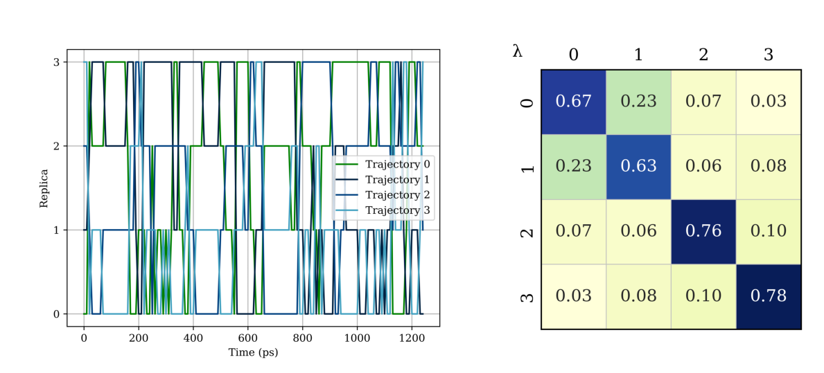
As shown in the replica-space trajectories in the left figure below, each replica was able to sample all different sets of states by exchanging coordinates with other replicas, indicating good sampling in the replica space. This decent sampling in the replica space is also reflected in the replica-space transition matrix in the right figure, where all tridiagonal elements are non-zero.

images = ['example_outputs/analysis/rep_trajs.png', 'example_outputs/analysis/rep_transmtx_allconfigs.png']
display_images_matplotlib(images, rows=1, widths=[60, 40], figsize=(12, 6))

4.2. State-space sampling

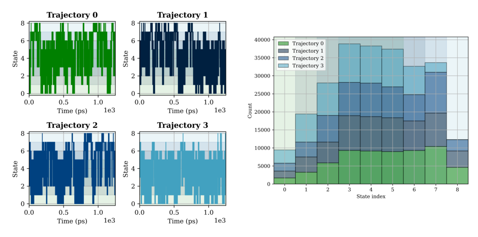
The state-space trajectories in the left figure below shows that each replica was able to sample all alchemical intermediate states, which requires not only replica-space transitions, but also state-space transitions facilitated by alchemical weights that flatten out the free energy surface along the alchemical direction. In the right figure, we show the visitation distribution in the state space, with contributions of visitation counts from different replicas shown in different colors. As some of the states can be accessed by multiple replicas, it is natural to not have a flat accumulate histgram here. In fact, the visitation count of each state should be proportional to the number of replicas that can access the state in an ideal case (i.e., each replica has an even sampling across all states).

images = ['example_outputs/analysis/state_trajs.png', 'example_outputs/analysis/state_hist.png']
display_images_matplotlib(images, rows=1)

Similarly, the efficient sampling in the state space is reflected by the state-space transition matrices of different continuous trajectories shown below. (Note that here we have one transition matrix for each replica.)

images = [f'example_outputs/analysis/traj_{i}_state_transmtx.png' for i in range(4)]
display_images_matplotlib(images, rows=2, figsize=(10, 10))

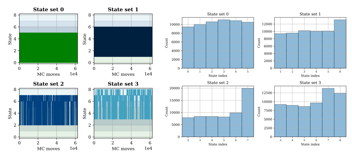
In addition to plotting continuous state-space trajectories, it could also be interesting to plot the time series of state visitation for different sets of states. That is, in the left figure below, each time series is contributed by different replicas at different times and the state vistation histogram for each state set is shown in the right figure. Note that ideally, the histograms on the right should be flat, but any \(N_\text{ratio}\) (highest count/lowest count) below 5 is generally acceptable for a short simulation like this one.

images = ['example_outputs/analysis/state_trajs_for_sim.png', 'example_outputs/analysis/state_hist_for_sim.png']
display_images_matplotlib(images, rows=1, figsize=(12, 6), widths=[45, 55])

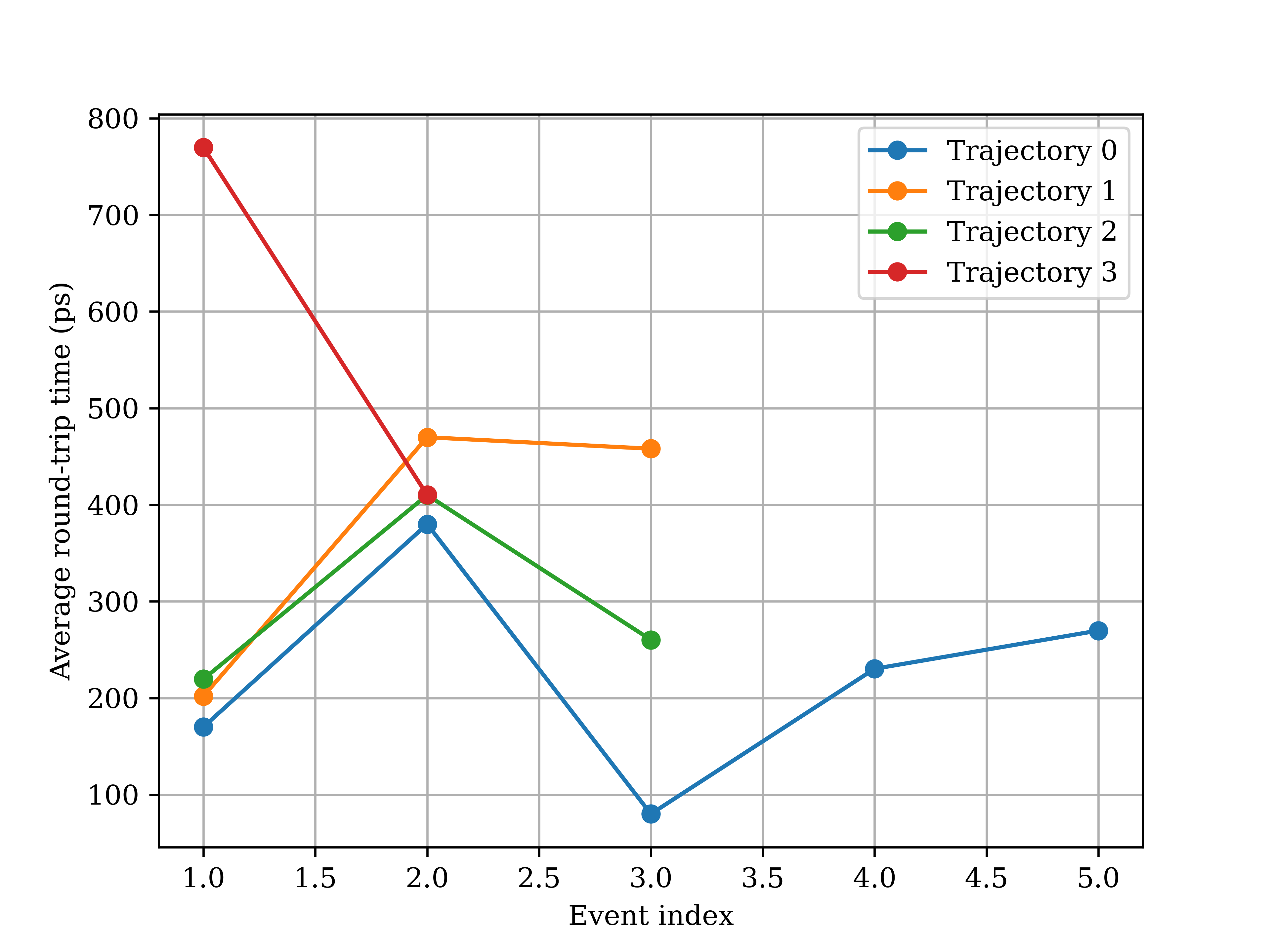
As shown in analyze_REXEE_log.txt, we have also calculated and plotted the time it takes for a replica to traverse the state space in either direction.

images = ['example_outputs/analysis/t_0k.png', 'example_outputs/analysis/t_k0.png']
display_images_matplotlib(images, rows=1)

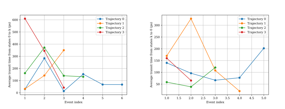
The sum of these two transit times is the round-trip time. A shorter state-space round-trip time generally indicates better sampling in the state space.

display(Image(filename='example_outputs/analysis/t_roundtrip.png', width=400))

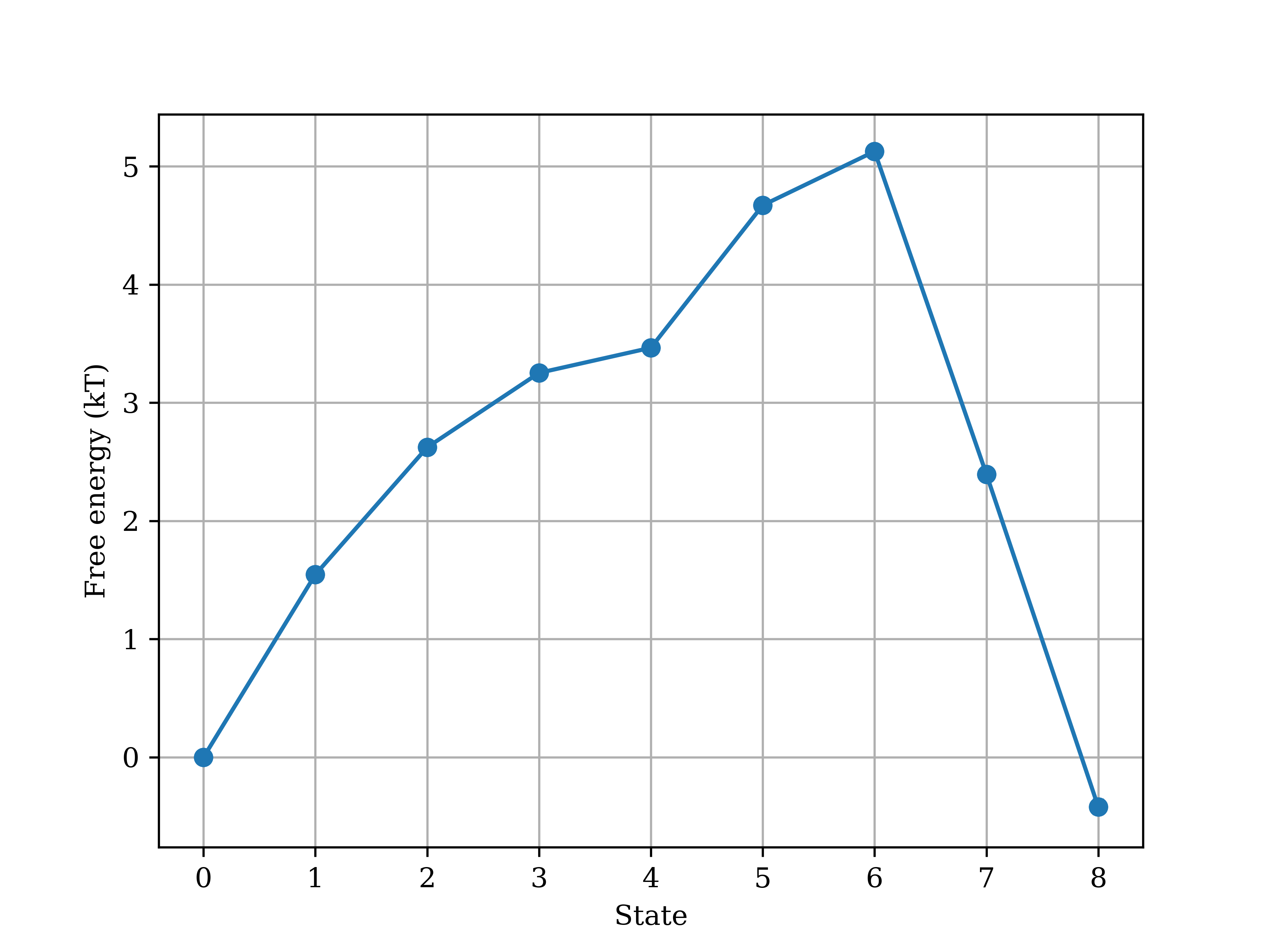
4.3. Free energy calculation

As shown in analyze_REXEE_log.txt, the solvation free energy of the toy molecule, which is the free energy difference between the coupled and decoupled states, was estimated as \(-0.42\pm0.60\) \(\mathrm{k_BT}\). Additionally, the free energy profile along the alchemical direction was also plotted, as shown below. The error bars werer plotted but are too small to be visible in the figure. Notably, the default protocol for truncating and decorrelating the dhdl data may not be optimal for a short simulation and can be case-dependent, so the uncertainty estimate in our example here may not be accurate. For more complicated systems with sufficient sampling, you may want to consider setting the parameter subsampling_avg to True in the input YAML file to dilute the effect of inaccurate estimation of truncation/decorrelation times for any replica, hence obtaining more reliable free energy estimates and their associated uncertainties.

display(Image(filename='example_outputs/analysis/free_energy_profile.png', width=400))

---

So this is the end of the tutorial! If you have any questions or suggestions about the tutorial, please feel free to file an issue on the GitHub repository of the package ensemble_md. We are happy to help you out! If you find the package ensemble_md useful for your research, please cite the following paper:

       Hsu, W. T., & Shirts, M. R. (2024). Replica Exchange of Expanded Ensembles: A Generalized Ensemble Approach with Enhanced Flexibility and Parallelizability. Journal of Chemical Theory and Computation. doi: 10.1021/acs.jctc.4c00484