Tutorial 2: Multi-topology REXEE (MT-REXEE) simulations
Note: This tutorial is still a work in progress. Some of the descriptions below may not yet be fully accurate or consistent with the provided example files — please double-check important details (e.g., simulation parameters) against params.yaml, expanded.mdp, and the other input files in this folder.

In this tutorial, we will demonstrate how one can use the different command-line interfaces (CLIs) implemented in the Python package ensemble_md to prepare, perform, and analyze a MT-REXEE simulation to estimate the solvation free energy of a toy molecule composed of 4 interaction sites. For a more comprehensive understanding, we strongly recommend reading our documentation on launching MT-REXEE simulations before starting
this tutorial. For the theory behind the MT-REXEE method, we recommend reading our JCTC paper or the theory section of our documentation.
To run this tutorial, you will need different setups depending on your computing environment:
You can simply click the “launch binder” badge above to run this tutorial on Binder without installing anything.
If you prefer to run this tutorial locally, either on you laptop, workstation, or an HPC cluster, you will need to install the following software:
GROMACS (version 2025.0 or later)
We recommend using GROMACS version 2025.0 or later in order to utilize the MDP option
init_histogram_countswhich will significantly increase the speed with which weights equilibrate.
ensemble_md (version 1.1.0 or later)
Additionally, you will need to have MPI launcher commands (e.g., mpirun or mpiexec) installed on your system to run the GROMACS simulations in parallel. You will need at least four CPU cores to run the simulation in this tutorial. (You can execute nproc in the terminal to check the number of CPU cores on your system.)
Notably, this tutorial assumes that you understand the basics of the expanded ensemble (EE) method and relevant simulation parameters in GROMACS. If not, we recommend reading the this tutorial or the following GROMACS documentation pages:
Relevant MDP parameters in GROMACS, especially the section of free energy calculation and the section of expanded ensemble calculations.
0. Background knowledge: Recommended Simulation Protocol
As in tutorial 1, this tutorial will only discuss the fixed-weight MT-REXEE simulation. Below we discuss a recommended protocol for getting to the fixed weight simulation stage.
Determine the optimal \(\lambda\) state spacing with independent expanded ensemble(EE) calculations.
We recommend that one performs independent short EE simulations for at least one transformation for which you plan to run MT-REXEE. In general if the transformations are varying a similar number of heavy atoms then the same \(\lambda\) state spacing will be sufficient for each.
If your set of simulations contains significantly different transformations then we recommend ensuring that your \(\lambda\) state spacing produces sufficient state overlap for each significantly different transformation.
Perform weight-updating MT-REXEE simulations.
The only difference between the set-up for weight-updating and fixed-weight MT-REXEE simulations is a few MDP parameters
Weight-updating:
lmc_weights_equil = wl-deltavs Fixed-weight:lmc_weights_equil = yesWeight-updating:
lmc_stats = wang-landauvs Fixed-weight:lmc_stats = noThe following MDP options should only be used for weight-updating simulations
wl_scale = ...wl_ration = ...init_wl_delta = ...weight_equil_wl_delta = ...
Perform fixed-weight MT-REXEE simulation.
Extract the equilibrated weights from the last iteration of the weight-updating MT-REXEE simulation and provide these with the MDP option
init_lambda_weights = ....This step will be discussed in detail below.
1. Preparing simulation inputs for a REXEE simulation
As mentioned in our documentation, running a REXEE simulation at least requires the following four input files:
One YAML file that specifies REXEE parameters.
NGROMACS GRO file of the system of interest.NGROMACS TOP file of the system of interest.One GROMACS MDP template for customizing MDP files for different replicas during the simulation.
The N is equal to the number of independent transformation you wish to perform with MT-REXEE. In the folder where this tutorial resides (docs/examples/tutorial_2 in the repository), you should find all these necessary input files, including params.yaml, A-B.gro, B-C.gro, C-D.gro, D-E.gro, E-F.gro, A-B.top, B-C.top, C-D.top, D-E.top, E-F.top, and expanded.mdp. Note that the file example_outputs.zip is not relevant until the third section
(Analyzing a MT-REXEE Simulation).
[1]:
!ls
A-B.gro  B-C.gro  C-D.gro  D-E.gro  E-F.gro  MT_REXEE.ipynb  water_and_ions.itp
A-B.itp  B-C.itp  C-D.itp  D-E.itp  E-F.itp  expanded.mdp
A-B.top  B-C.top  C-D.top  D-E.top  E-F.top  params.yaml
The MDP template expanded.mdp can be inspected that it adopts common/typical settings for a fixed-weight EE simulation, since here our goal is to set up a fixed-weight REXEE simulation. In the MDP template, we define 7 alchemical intermediate states for each of the 5 transformations being performed here. To enable correct parsing of the MDP file the number of states for each transformation should be equilivalent, but the values may be different. In this example we use the same
\(\lambda\) state spacing for each transformation.
During the REXEE simulation, customized MDP files will be generated for different replicas such that the MDP file for each replica only considers the set of states that the replica is constrained to. Notably, the weights specified via the MDP parameter init_lambda_weights were obtained from a weight-updating MT-REXEE simulation.
Now, with these three GROMACS inputs prepared, let’s briefly review the input YAML file that specifies MT-REXEE parameters. (For detailed information about all possible parameters that can be specified in the YAML file, please refer to our documentation.)
[2]:
!cat params.yaml
n_sim: 5                     # Number of replica simulations
n_iter: 1000                 # Number of iterations
s: 7                        # Shift in λ ranges [e.g. s = 2 if λ_2 = [2, 3, 4] & λ_3 = [4, 5, 6]]
nst_sim: 20000               # Number of simulation steps for each homogeneous replica
proposal: 'random_range'
mdp: 'expanded.mdp'
add_swappables: [[6, 7], [13, 14], [20, 21], [27, 28]]
n_ckpt: 25
N_cutoff: -1
w_combine: False    # The method for combining weights. Choices include "None" [unspecified], exp_avg, ...
runtime_args: {'-ntomp': '4', '-ntmpi': '1'}
grompp_args: {'-maxwarn': '2'}
gro: ['A-B.gro', 'B-C.gro', 'C-D.gro', 'D-E.gro', 'E-F.gro']
top: ['A-B.top', 'B-C.top', 'C-D.top', 'D-E.top', 'E-F.top']
resname_list: ['A2B', 'B2C', 'C2D', 'D2E', 'E2F']
swap_rep_pattern: [[[0,1],[1,0]], [[1,1],[2,0]], [[2,1],[3,0]], [[3,1],[4,0]]]
gmx_executable: 'gmx'
verbose: True
modify_coords: 'default'

msm: False
free_energy: True
df_spacing: 1
df_method: "MBAR"
err_method: "propagate"
n_bootstrap: 50
seed : null
As a minimum working example, this YAML file only specifies the compulsory simulation parameters and adopts default values for all optional parameters, except that runtime_args is specified to run each EE replica using one thread (-nt 1) for a reasonable simulation performance. Notably, Binder should have 72 cores by default (as can be checked by nproc), but using -nt 1 is much faster than using other values for this toy system. If you are not using Binder but your own local
machine or an HPC cluster, you may want to try out other -nt values to ensure reasonable performance.
In our case, we will run a REXEE simulation composed of 4 replicas, with each replica performed with one thread (-nt 1). With the total number of states as 9 and a state shift of 1, this means that replicas 0, 1, 2, 3 are constrained to sampling states 0-5, 1-6, 2-7, and 3-8, respectively. The simulation will attempt to swap coordinates between replicas every 500 integration steps, and perform 5 iterations in total. (Note that generally we need a much larger number of iterations. Here we use
a very small value just for demonstration purposes.)
If you are interested in trying out other numbers of replicas or state shifts given 9 alchemical intermediate states, you can use the CLI explore_REXEE to enumerate all possible REXEE configurations.
2. Performing a MT-REXEE Simulation
Performing the MT-REXEE simulation is simply completed by running the command: mpirun -np x run_REXEE -y input.yaml Where x is equal to the number of separate simulations you wish to run. Below is the text of an example bash script to run a MT-REXEE simulation.
[3]:
!cat MTREXEE.sh
#!/bin/bash

#SBATCH --nodes 1
#SBATCH --partition=amilan
#SBATCH --ntasks=20
#SBATCH --job-name=tutorial
#SBATCH --qos=normal
#SBATCH --time=03:00:00
#SBATCH --output=tutorial.out

source /projects/anfr8476/pkgs/gromacs-2022.5-wl/bin/GMXRC
ml gcc
ml openmpi/5.0.6

conda activate EEXE

mpirun -np 5 run_REXEE -y params.yaml

mpirun -np 5 analyze_REXEE -y params.yaml
3. Analyzing a MT-REXEE Simulation
See the analyzing a MT-REXEE simulation section in tutorial 1 for a detail of all outputs. Below we will just consider the details of MT-REXEE specific outputs.
[8]:
!unzip example_outputs.zip > /dev/null 2>&1
[4]:
import gc
import matplotlib.pyplot as plt
import matplotlib.image as image
from IPython.display import display, Image

def display_images_matplotlib(images, widths=None, figsize=(10, 5), rows=1, titles=None):
    """
    Display a list of images in a grid using Matplotlib with specified widths.

    Parameters
    ----------
    images : List[str]
        List of image paths.
    widths : List[float]
        A list containing the width of each image as a percentage of the total width. Must add up to 100.
    figsize : tuple
        Size of the entire figure (width, height).
    rows : int
        Number of rows in the grid.
    titles : List[str]
        List of titles for each image. If None, no titles will be displayed.
    """
    cols = len(images) // rows + int(len(images) % rows != 0)

    if widths is None:
        widths = [100 / len(images) for _ in images]
    else:
        assert sum(widths) == 100, "The widths must add up to 100."

    fig, axes = plt.subplots(rows, cols, figsize=figsize, gridspec_kw={'width_ratios': widths[:cols]})
    axes = axes.flatten()

    for i, (img_path, ax) in enumerate(zip(images, axes)):
        img = image.imread(img_path)
        ax.imshow(img)
        ax.axis('off')
        if titles is not None:
            ax.set_title(titles[i])

    # Hide any remaining empty subplots
    for ax in axes[len(images):]:
        ax.axis('off')

    plt.tight_layout()
    plt.show()
    plt.close(fig)  # Close the figure to release memory
    gc.collect()  # Run garbage collection to free up memory as Binder only has 2 GB of RAM
3.1. Replica-space sampling
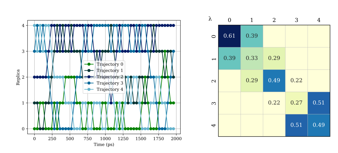
Analyzing replica swapping is slightly different for a MT-REXEE simulation because we are also analyzing swaps between different topologies. Each simulation samples 7 alchemical states corresponding to a given transformation and so for every 7 alchemical states you are sampling a different transformation. This is a short example and thus only one round-trip is sampled in simulation replica 3 as quantified in roundtrip_times.csv.
[10]:
images = ['analysis/rep_trajs.png', 'analysis/rep_transmtx_allconfigs.png']
display_images_matplotlib(images, rows=1, widths=[60, 40], figsize=(12, 6))
[11]:
!cat analysis/roundtrip_times.csv
,Sim,Round Trip Time
0,3,696.4000000000001
3.2. Free Energy Estimates
The code will also compute the relative free energy for each transformation and the error in units kcal/mol.
[12]:
!cat analysis/FE_estimates.csv
,Transformation,FE Estimate,FE Error
0,A2B,14.374228379123714,0.26737398764600245
1,B2C,2.3928813271047034,0.24983640186414527
2,C2D,9.056942986915711,0.10837506024641683
3,D2E,3.108082460752591,0.15299665759636027
4,E2F,-12.585227286341368,0.11339380834329797
3.3. File concatenation
The final added analysis functionality is concatenating the trajectory and xvg files from all replicas. Running long MT-REXEE simulations can produce thousands of files which are not practical to store long-term. We can reduce the size of the output files produced by simply concatenating the trajectories and xvg files into a single file for each replica. The concatenated trajectories can be found in the folder analysis/traj and the energy files can be found in the analysis folder.
[13]:
!ls analysis/traj
sim0_concat.xtc  sim2_concat.xtc  sim4_concat.xtc
sim1_concat.xtc  sim3_concat.xtc
[17]:
!head -n 50 analysis/sim_0.xvg
# This file was created Sun Jan 25 11:52:49 2026
# Created by:
#                    :-) GROMACS - gmx mdrun, 2022.5-dev (-:
#
# Executable:   /projects/anfr8476/pkgs/gromacs-2022.5-wl/bin/gmx
# Data prefix:  /projects/anfr8476/pkgs/gromacs-2022.5-wl
# Working dir:  /projects/anfr8476/EEXE/tutorial/sim_0/iteration_0
# Command line:
#   gmx mdrun -s sys_EE.tpr -ntomp 4 -ntmpi 1
# gmx mdrun is part of G R O M A C S:
#
# Getting the Right Output Means no Artefacts in Calculating Stuff
#
@    title "dH/d\xl\f{} and \xD\f{}H"
@    xaxis  label "Time (ps)"
@    yaxis  label "dH/d\xl\f{} and \xD\f{}H (kJ/mol [\xl\f{}]\S-1\N)"
@TYPE xy
@ subtitle "T = 300 (K) "
@ view 0.15, 0.15, 0.75, 0.85
@ legend on
@ legend box on
@ legend loctype view
@ legend 0.78, 0.8
@ legend length 2
@ s0 legend "Thermodynamic state"
@ s1 legend "Total Energy (kJ/mol)"
@ s2 legend "dH/d\xl\f{} coul-lambda = 0.0000"
@ s3 legend "dH/d\xl\f{} vdw-lambda = 0.0000"
@ s4 legend "dH/d\xl\f{} bonded-lambda = 0.0000"
@ s5 legend "\xD\f{}H \xl\f{} to (0.0000, 0.0000, 0.0000)"
@ s6 legend "\xD\f{}H \xl\f{} to (0.1000, 0.1000, 0.1000)"
@ s7 legend "\xD\f{}H \xl\f{} to (0.3000, 0.3000, 0.3000)"
@ s8 legend "\xD\f{}H \xl\f{} to (0.6000, 0.6000, 0.6000)"
@ s9 legend "\xD\f{}H \xl\f{} to (0.7000, 0.7000, 0.7000)"
@ s10 legend "\xD\f{}H \xl\f{} to (0.8500, 0.8500, 0.8500)"
@ s11 legend "\xD\f{}H \xl\f{} to (1.0000, 1.0000, 1.0000)"
@ s12 legend "pV (kJ/mol)"
0.0000    0 -22122.805 347.00275 -6.0445342 0.27468288 0.0000000 26.156464 56.833501 93.372061 116.35304 225.14488 2522.7875 1.2356462
0.2000    0 -22189.439 214.88879 -5.3762889 4.2629437 0.0000000 18.872757 45.444998 69.765013 77.536667 98.394983 177.18662 1.2289184
0.4000    0 -22194.668 117.93085 -5.2653904 3.7813795 0.0000000 10.688006 27.839856 50.456709 60.305595 83.898573 137.06987 1.2259645
0.6000    1 -22203.967 75.140091 6.0182362 0.96916145 -8.4235077 0.0000000 16.160481 48.761357 69.535536 136.09242 401.34042 1.2287536
0.8000    1 -22183.102 101.17058 2.0457270 1.6275749 -11.200690 0.0000000 19.106085 52.523059 75.639188 177.22709 1656.4120 1.2278885
1.0000    1 -22168.238 79.165504 -6.9147930 0.64437413 -7.8168343 0.0000000 12.946592 31.793526 42.758798 85.035059 372.64980 1.2264318
1.2000    0 -22171.555 345.90173 -13.892157 6.3481512 0.0000000 24.893316 50.232685 65.397788 67.187025 68.501146 72.123709 1.2277149
1.4000    0 -22150.359 255.60376 -0.064769983 1.6827195 0.0000000 20.074296 44.801702 78.720641 98.378429 166.61731 615.54077 1.2282300
1.6000    0 -22108.109 146.93002 2.8224769 9.3693266 0.0000000 14.420737 38.568611 83.178096 111.13355 201.19222 589.33768 1.2300092
1.8000    0 -22142.254 251.36328 1.2828643 1.3996387 0.0000000 20.471506 47.278047 86.273217 110.32509 202.37016 1102.6249 1.2304920
2.0000    0 -22174.004 196.71042 -3.6515193 5.0444965 0.0000000 16.647373 39.150289 65.938763 78.725749 118.65153 307.03463 1.2314249
2.2000    0 -22116.258 98.408157 -1.8035878 10.069950 0.0000000 10.283106 30.229422 75.646227 107.89390 219.29637 712.98939 1.2357938
2.4000    1 -22109.305 80.721062 1.5316250 5.8552127 -9.2031419 0.0000000 16.458660 43.697230 58.969626 107.78196 341.39230 1.2387666