1. Basic idea
Replica exchange of expanded ensembles (REXEE) [Hsu2024] integrates the core principles of replica exchange (REX) [Sugita1999] and expanded ensemble (EE) [Lyubartsev1992] method. Specifically, a REXEE simulation performs multiple replicas of EE simulations in parallel and periodically exchanges coordinates between replicas. Each replica samples a different but overlapping set of alchemical intermediate states to collectively sample the space between the fully coupled (\(\lambda=0\)) and decoupled states (\(\lambda=1\)). By design, the REXEE method decorrelates the number of replicas from the number of states, enhancing the flexibility in replica configuration and allowing a large number of intermediate states to be sampled with significantly fewer replicas than those required in the Hamiltonian replica exchange (HREX) method [Sugita2000]. By parallelizing replicas, the REXEE method also reduces the simulation wall time compared to the EE method. More importantly, such parallelism sets the stage for more complicated applications, especially one-shot free energy calculations that involve multiple topologies, such as serial mutations or scaffold-hopping transformations.
In the following sections, we will briefly cover the theory behind the REXEE method, from its configuration, state transitions, proposal schemes, weight combination schemes, to data analysis. For more details, please refer to our paper [Hsu2024].

Fig. 1 Figure 1. Schematic representation of the REXEE method, with the four configurational parameters annotated. In a REXEE simulation, the coordinates of replicas of EE simulations are periodically exchanged. \({\bf A}_1\), \({\bf A}_2\), \({\bf A}_3\), and \({\bf A}_4\) denote the sets of states different replicas are sampling.
The REXEE architecture can easily lend itself to performing several alchemical transformations in the parallel simulation rather than decomposing the alchemical states between the parallel simulations as is utilized in the REXEE implementation. The mulitple topology replica exchange of expanded ensemble (MT-REXEE) method allows for parallel transformation with overlapping end steps to engage in conformational swaps to increase conformational sampling [Friedman2025]. Any transformation within the trsnformation network with a common end state can engage in conformational swap and increase conformational sampling. This method is ideal for systems which have high free energy barriers present for only a subset of ligands to be evaluated.
2. REXEE configuration
Here we consider a REXEE simulation composed of \(R\) parallel replicas of expanded ensembles, each of which is labeled as \(i=1, 2, ..., R\). These \(R\) replicas are restricted to sampling \(R\) different yet overlapping sets of states (termed state sets) labeled by \(m\) as \({\bf A}_1\), \({\bf A}_2\), …, \({\bf A}_R\), which collectively sample \(N\) alchemical intermediate states in total, with \(N > R\). Additionally, we define \(s_i \in \{1, 2, ..., N\}\) as the index of the state currently sampled by the \(i\)-th replica. For a replica \(i\) sampling state set \({\bf A}_m\), \(s_i\) is additionally constrained such that \(s_i \in {\bf A}_m\). Importantly, the fact that \(s_i\) takes values in \(\{1, 2, ..., N\}\) and \(N>R\) implies a many-to-one relationship between the replica index \(i\) and the state index \(s_i\), as a certain state may be sampled by multiple replicas. This is in contrast to the one-to-one relationship between the replica index \(i\) and the state set index \(m\), which ensures that each replica is associated with one unique state set.
Importantly, a valid REXEE configuration only requires overlapping state sets and is not restricted to one-dimensional grids,
the same number of states for all replicas, nor sequential state indices within the same state sets. For example, Fig. 2 shows cases where
intermediate states are characterized by more than one thermodynamic variable (panels A and B), where different state sets
have different numbers of states (panels C), and where the state indices are not consecutive within the same state sets (panels A and C).
Still, the most common case is where the intermediate states are defined in a one-dimensional space, with consecutive state indices within
the same state set (e.g., the case in Fig. 1). In a REXEE simulation with such a configuration, a state shift \(\phi\) between adjacent
state sets can be defined to indicate to what extent the set of states has shifted along the alchemical coordinate. Depending on whether all replicas
have the same number of states and whether or not the state shift is consistent between all adjacent state sets, a REXEE simulation can be either
homogeneous or heterogeneous. Currently, ensemble_md has only implemented the homogeneous REXEE method with one-dimensional alchemical intermediate
states defined sequentially in each state set.

Fig. 2 Figure 2. Different possible replica configurations of a REXEE simulation, with each state represented as a grid labeled by the number in its center and characterized by different Hamiltonians and/or temperatures. Different state sets are represented as dashed lines in different colors. Note that the temperature \(T\) and Hamiltonian \(H\) can be replaced by other physical variables of interest, such as pressure or chemical potential.
As shown in Fig. 1, a homogeneous REXEE simulation that samples sequential one-dimensional states can be configured by the following four parameters:
\(N\): The total number of intermediate states
\(R\): The total number of replicas
\(n_s\): The number of states per replica
\(\phi\): The state shift between adjacent state sets
These four configurational parameters are related via the following relationship:
For example, the configuration of the REXEE simulation shown in Fig. 1 can be expressed as \((N, R, n_s, \phi) = (9, 4, 6, 1)\). Importantly, the total
number of states \(N\) does not have to be equal to the number of replicas \(R\) in the REXEE method. In fact, it is shown in the Supporting Information of
our paper [Hsu2024] that for a REXEE simulation simulation sampling any number of replicas, there exists at least one valid REXEE
configuration, allowing much higher flexibility in replica configuration compared to traditional replica exchange methods – once the number of replicas
is decided, typically as a factor of the number of available cores, the total number of states can be arbitrary. In our Supporting Information,
we also show that solving Equation (1) with a few additional constraints allows efficient enumeration of all possible REXEE configurations. In ensemble_md,
this enumeration is implemented in the command line interface (CLI) command explore_REXEE, as elaborated in 1.1. CLI explore_REXEE.
3. State transitions in REXEE simulations
In a REXEE simulation, state transitions occur at both the intra-replica and inter-replica levels. Within each replica of expanded ensemble simulation,
transitions between alchemical states within the state set and the detailed balance conditions are governed by the selected algorithm in the expanded ensemble simulation
(i.e., the value of the GROMACS MDP parameter lmc-stats-move in our implementation). Still, to ensure that probability influx and outflux are equal for each set of states,
the detailed balance condition at the intra-replica level must be satisfied.
Mathematically, we consider replicas \(i\) and \(j\) that sample the state sets \({\bf A}_m\) and \({\bf A}_n\), respectively. To swap replicas \(i\) and \(j\), the state sampled by replica \(i\) at the moment, denoted as \(s_i \in {\bf A}_m\), must fall within the state set \({\bf A}_n\) that is to be swapped, and vice versa. In this case, we call that these replicas \(i\) and \(j\) are swappable, and we express the exchange of coordinates \(x_i\) and \(x_j\) between these two replicas as
with \(x^i_m \equiv (x_i, {\bf A}_m)\) meaning that the \(i\)-th replica samples the \(m\)-th state set with the coordinates \(x_i\). Mathematically, the list of swappable pairs \(\mathcal{S}\) can be defined as the set of replica pairs as follows:
As discussed in the Supporting Information of the paper [Hsu2024], the most straightforward way to derive the acceptance ratio that satisfies the intra-replica detailed balance condition is to assume symmetric proposal probabilities, which can be easily achieved by the design of the used proposal scheme. (See 4. Proposal schemes for more details.) Under this assumption, the acceptance ratio of swapping the coordinates \(x_i\) and \(x_j\) between replicas \(i\) and \(j\) can be expressed as
where
In Equation (5), \(u_{s_i}(x_j)\) and \(u_{s_j}(x_i)\) are the reduced potentials of the states \(s_i\) and \(s_j\) evaluated at the coordinates \(x_j\) and \(x_i\), respectively.
4. Proposal schemes
In this section, we discuss proposal schemes available in the current implementation of the package ensemble_md,
each of which has a symmetric proposal probability. These proposal schemes can be specified via the option proposal in the input YAML file (e.g., params.yaml)
for running a REXEE simulation. For more details about the input YAML file, please refer to 3. Input YAML parameters.
4.1. Single exchange proposal scheme
The single exchange proposal scheme randomly draws a pair of replicas from the list of swappable pairs \(\mathcal{S}\) defined in (3), with each pair in the list having an equal probability to be drawn. In this case, the proposal probability can be expressed as follows:
In our implementation in ensemble_md, this method can be used by setting proposal: 'single' in the input YAML file.
4.2. Neighbor exchange proposal scheme
In the neighbor exchange proposal scheme implemented in ensemble_md (which is enabled by setting proposal: 'neighbor' in the input YAML file),
we add a constraint to the swappable pairs defined in Equation (3) such that the swappable pairs consist exclusively of neighboring replicas,
with each pair having an equal probability to be drawn. Formally, the proposal probability in this case can be expressed as
follows:
where
4.3. Exhaustive exchange proposal scheme
As opposed to the single exchange or neighbor exchange proposal schemes, one can propose
multiple swaps within an exchange interval to further enhance the mixing of replicas. In ensemble_md,
one available method is the exhaustive exchange proposal scheme, which can be enabled by setting proposal: 'exhaustive' in the input YAML file.
As detailed in Algorithm 1 below, the exhaustive exchange proposal scheme operates similarly to the single exchange proposal scheme, but
exhaustively traverses the list of swappable pairs while updating the list by eliminating any pair involving replicas that
appeared in the previously proposed pair, ensuring symmetric proposal probabilities. Intuitively, the exhaustive exchange proposal
scheme leads to more efficient state-space and replica-space sampling than the other two
proposal schemes, as it potentially allows for more exchanges to occur within an exchange interval.

5. Correction schemes
For weight-updating REXEE simulations, we experimented with a few correction schemes that aim to improve the convergence of the alchemical weights.
These correction schemes include weight combination and histogram correction schemes, which can be enabled by setting
w_combine: True and hist_corr: True in the input YAML file, respectively. While there has not been evidence showing that these correction schemes could improve the
weight convergence in REXEE simulations (as discussed in our paper [Hsu2024]), we still provide these options for users to experiment with.
In the following sections, we elaborate on the details of these correction schemes.
5.1. Weight combination
In contrast to other generalized ensemble methods such as EE or HREX methods, the REXEE method possesses overlapping states, i.e.,
the states that fall within the intersection of at least two state sets and are therefore accessible by multiple replicas. To leverage the statistics of
these overlapping states, we could combine the alchemical weights of these states across replicas before
initializing the next iteration. The hypothesis is that such on-the-fly modifications to the weights could potentially
accelerate the convergence of the alchemical weights and provide a better starting point for the subsequent production phase.
Noting that there are various ways to combine the weights of overlapping states across replicas, the simple approach we have implemented in ensemble_md
is to simply calculate the average of the weight differences accessible by multiple replicas, and reassign weights based on these averages to the overlapping states.
This average can be either a simple average or an inverse-variance weighted average, which is less sensitive to the presence of outliers in the weight differences.
Mathematically, we write the weight difference between the states \(s\) and \(s+1\) in replica \(i$\) as \(\Delta g_{(s, s+1)}^i=g^i_{s+1}-g^i_{s}\),
and the set of replicas that can access both \(s\) and \(s+1\) as \(\mathcal{Q}_{(s, s+1)}\). Then, for the case where the inverse-variance weighting is used,
we have the averaged weight difference between \(s\) and \(s+1\) as:
with its propagated error being
where \(\sigma^k_{(s, s+1)}\) is the standard deviation calculated from the time series of \(\Delta g^{k}_{(s, s+1)}\) since the last update of the Wang-Landau incrementor in the EE simulation sampling the \(k\)-th state set. For a more detailed demonstration of weight combinations, please refer to the example below.
Here we consider the following sets of weights
as an example, with X denoting a state not present in the state set:
State       0         1         2         3         4         5
Rep A       0.0       2.1       4.0       3.7       X         X
Rep B       X         0.0       1.7       1.2       2.6       X
Rep C       X         X         0.0       -0.4      0.9       1.9
As shown above, the three replicas sample different but overlapping states. Now, our goal is to
For state 1, combine the weights arcoss replicas 1 and 2.
For states 2 and 3, combine the weights across all three replicas.
For state 4, combine the weights across replicas 1 and 2.
That is, we combine weights arcoss all replicas that sample the state of interest regardless of
which replicas are swapping. The outcome of the whole process should be three vectors of modified
alchemical weights, one for each replica, that should be specified in the MDP files for the next iteration.
Below we elaborate on the details of each step carried out by our method implemented in ensemble_md.
First, we calculate the weight differences as shown below, which can be regarded as rough estimates of free energy differences between the adjacent states.
States      (0, 1)    (1, 2)    (2, 3)    (3, 4)    (4, 5)
Rep 1       2.1       1.9       -0.3       X        X
Rep 2       X         1.7       -0.5       1.4      X
Rep 3       X         X         -0.4       1.3      1.0
Note that to calculate the difference between, say, states 1 and 2, from a certain replica,
both these states must be present in the alchemical range of the replica. Otherwise, a free
energy difference can’t not be calculated and is denoted with X. Then, for the weight differences that are available in more than 1 replica, we take the simple
average of the weight differences. That is, we have:
States      (0, 1)    (1, 2)    (2, 3)    (3, 4)    (4, 5)
Final       2.1       1.8       -0.4      1.35      1.0
Assigning the first state as the reference that has a weight of 0, we have the following profile:
Final g 0.0 2.1 3.9 3.5 4.85 5.85
Notably, In our implementation in ensemble_md (or more specifically, the function combine_weights in the class ReplicaExchangeEE in replica_exchange_EE),
inverse-variance weighted averages can be used instead of simple averages used above, in which case uncertainties of the input weights (e.g., calculated as the standard
deviation of the weights since the last update of the Wang-Landau incrementor) are required.
Finally, we need to determine the vector of alchemical weights for each replica. To do this, we just shift the weight of the first state of each replica back to 0. As a result, we have the following vectors:
State       0           1            2            3            4            5
Rep 1       0.0         2.1          3.9          3.5          X            X
Rep 2       X           0.0          1.8          1.4          2.75         X
Rep 3       X           X            0.0          -0.4         0.95         1.95
As a reference, here are the original weights:
State       0           1            2            3            4            5
Rep 1       0.0         2.1          4.0          3.7          X            X
Rep 2       X           0.0          1.7          1.2          2.6          X
Rep 3       X           X            0.0          -0.4         0.9          1.9
Notably, taking the simple average of weight differences/free energy differences is equivalent to taking the geometric average of the probability ratios.
5.2. Weight correction
In the weight combination method shown above, we frequently exploited the relationship \(g(\lambda)=f(\lambda)=-\ln p(\lambda)\). However, this relationship is true only when the histogram of state visitation is exactly flat, which rarely happens in reality. To correct this deviation, we can convert the difference in the histogram counts into the difference in free energies. This is based on the fact that the ratio of histogram counts is equal to the ratio of probabilities, whose natural logarithm is equal to the free energy difference of the states of interest. Specifically, we have:
where \(g'_k\) is the corrected alchemical weight of state \(k\), and \(N_{k-1}\) and \(N_k\) are the histogram counts of states \(k-1\) and \(k\), respectively.
5.3. Histogram correction
In our experiment, we have also tried applying histogram corrections upon weight combination across replicas to
correct the effect that the targeting distribution is a function of time. The idea is to leverage the more
reliable statistics we get from the overlapping states. In a limiting case where we have two weight-updating
EE simulations sampling the same set of states, the way we take full advantage of all the samples collected
in two simulations is to consider the histogram of both simulations and base the flatness criteria on the
sum of the histograms from both simulations, in which case the weights should then equilibrate faster
than a single weight-updating EE simulation. Click the example below to see a more detailed demonstration/derivation
of the histogram correction approach implemented in ensemble_md.
Here, we consider replicas A and B sampling states 0 to 4 and states 1 to 5, respectively. At time \(t\), these two replicas have the following weights for their state sets.
Alchemical weights

State         0         1         2         3         4         5
Rep A         0         4.00      10.69     12.18     12.52     X
Rep B         X         0         5.15      7.14      8.48      8.16
And the histogram counts at time \(t\) are as follows
Histogram counts
State         0         1         2         3         4         5
Rep A         416       332       130       71        61        X
Rep B         X         303       181       123       143       260
During weight combination, for states 1 and 2, we calculate the following average weight difference:
Let \(\Delta f'_{21}=\ln\left(\frac{N_1'}{N_2'}\right)\). We then have
In synchronous REXEE simulations, each replica should have the same total amount of counts, so the normalization constant for replicas A and B are the same, i.e., \(p^A_1 = N^A_1/N\), \(p^B_1 = N^B_1/N\), … etc. Therefore, we have
That is, the ratio of corrected histogram counts should be the geometric mean of the ratios of the original histogram counts. Using the numbers above, we calculate the ratios of histogram counts for all neighboring states. That is, for states accessible by multiple replicas, we calculate the geometric mean of the values of \(N_{i+1}/N_i\) from different replicas. Otherwise, we simply calculate \(N_{i+1}/N_i\).
States     (0, 1)     (1, 2)       (2, 3)       (3, 4)       (4, 5)
Final       0.798      0.484        0.609        0.999       1.818
Note that given \(N_1\), we can get \(N_2\) by calculating \(N_1 \times \frac{N_2}{N_1}\) and get \(N_2\) by calculating \(N_1 \times \frac{N_2}{N_1} \times \frac{N_3}{N_2}\) and so on. So the histogram counts of the whole set of states would be as follows:
Final N 416 332 161 98 98 178
The above distribution can be used to derive the distribution for each state set easily:
States    0     1     2     3     4     5
Rep A     416   332   161   98    98
Rep B     X     332   161   98    98    178
5.3. Our experience with the correction schemes
As per our experiments with the correction schemes (also partly discussed in our paper [Hsu2024]), here are some interesting observations about the correction schemes:
Generally, the application of weight combination schemes would lengthen the weight convergence time for a weight-updating REXEE simulation, without necessarily converging to more accurate weights, as compared to running a weight-updating EE simulation for each state set.
Interestingly, in terms of the weight convergence time and the weight accuracy, here is the ranking of the performance of different combinations of the correction schemes, with the best performance listed first:
No correction schemes at all, i.e., weight-updating EE simulation for each state set.
Weight combination with simple averages + histogram correction
Weight combination with simple averages
Weight combination with inverse-variance weighted averages
We reason these observations that combining weights does not improve convergence is because the exchanges of coordinates between replicas have already caused each replica to visit all of the configurations that started with different replicas, and thus have “seen” the different configurations and incorporated them into the accumulated weights. Therefore, additionally combining weights across replicas may not provide any additional advantage. In addition, small changes in weights can drastically affect sampling, as state probabilities are exponential in the free energy differences between states. If one of the weights being combined is particularly bad, it will disrupt sampling for the other weights, and will therefore lower the convergence rate. For more details about the experiments, please refer to our paper [Hsu2024].
6. Free energy calculations
The free energy calculation protocol of the REXEE method is basically the same as those for the EE and HREX methods.
Specifically, for each state set in a fixed-weight REXEE simulation, we concatenate the trajectories from all replicas, truncate the non-equilibrium
region, and then decorrelate the concatenated data. Then, for each replica in the fixed-weight REXEE simulation, one can use
free energy estimators such as TI, BAR, and MBAR to calculate the alchemical free energies for different state sets.
For the overlapping states, one can then use Equations (9) and (10) to calculate the mean of the associated free energy differences
\(\overline{\Delta G_{(s, s+1)}}\) and the accompanying propagated error \(\delta_{(s, s+1)}\), with \(\Delta g^k_{(s, s+1)}\)
replaced by \(\Delta G^k_{(s, s+1)}\), the free energy difference computed by the chosen free energy estimator. In this context,
\(\sigma^k_{(s, s+1)}\) used in Equations (9) and (10) should be the uncertainty associated with \(\Delta G^k_{(s, s+1)}\)
calculated by the estimator. In ensemble_md, this has been implemented in the function calculate_free_energy() in analyze_free_energy.
7. MT-REXEE Coordinate Modification
The MT-REXEE method requires that coordinates for the non-matching dummy atoms between two transformations must be reconstructed in order to swap coordinates.
The default cordinate modification function provided within this package can be selected by adding modify_coords: default to your input YAML file.
Alternatively, a custom function can be provided by the user. For this explanation we will be using the defualt function to perform a swap between a simulation
which features molecule A and a simulation which features molecule B. We first determine which atoms are missing between determines all atoms which are present
in molecule A but not in B and vice versa. By definition these atoms must be dummy atoms in their fully non-coupled state when the swap is performed. These
missing atoms are then broken up by functional group to create several missing R groups. The alignment is then performed individually for each missing R group
as shown in Figure ?. This will provide coordinates for the R groups unique to molecule B consistant with the structure of the common atoms in molecule A and vice
versa. This allows new GRO files to be written and the next iteration to be perfomed.
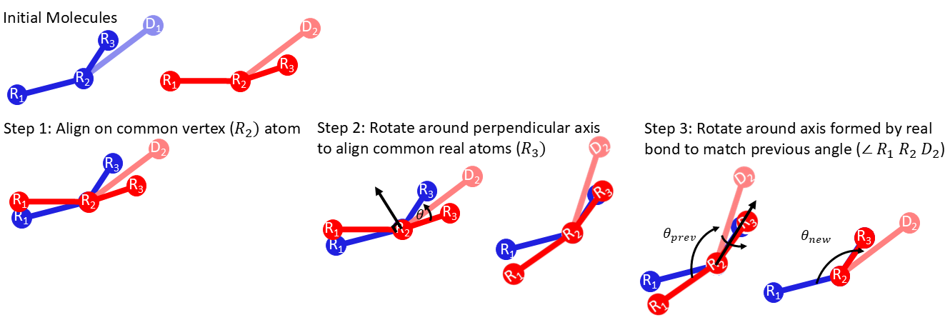
Fig. 3 Figure 3. A diagram of the method in which missing atoms coordinates are reconstructed during the conformational swaps. In this example, we construct atoms for the red dummy group (\(D_{2, red}\)) for the blue molecule configuration. The blue molecule may sometimes contain alternate dummy groups (\(D_{1, blue}\)) which will not show up in the new configuration, so these are ignored for the alignment protocol.